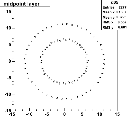
The following plots look at a single column of ministrips in the first
plane ('layer 9') of the DOE detector (type 1 = cone, type 2 = flat), using
central gold-gold events, with the event vertex at z=0.
This is the part of the detector where occupancies are the highest.
(files /phenix/data07/hubert/pythia2/
auau/ancsvx_auau_typeX.root,
where X is 1-4)
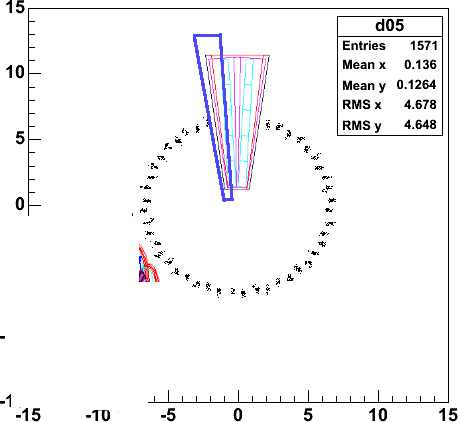
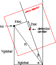
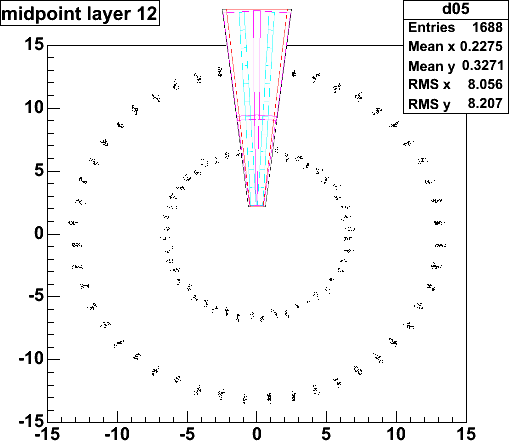
I look at the smallest readout unit, a single column of ministrips, serviced
by 5 readout chips (outlined in dark blue in the figure).
| 
|
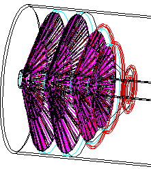
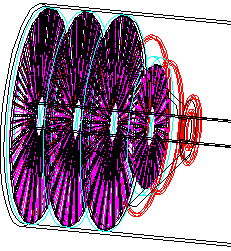
| The plots are for these configurations: type 1 is the lampshades,
type 2 is the flat planes
| 
| 
|
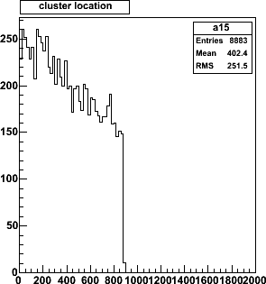
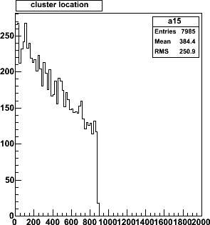
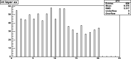
| Track distribution vs strip number. The inner
silicon is 6.6 cm high, so that there are 880 75-um strips. There is
a small difference between the two configurations due to the plane's angles.
| 
| 
|
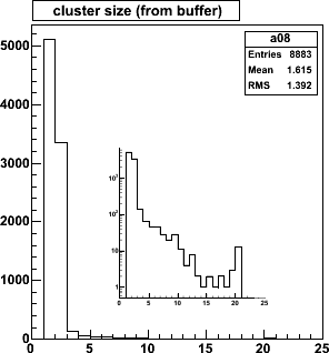
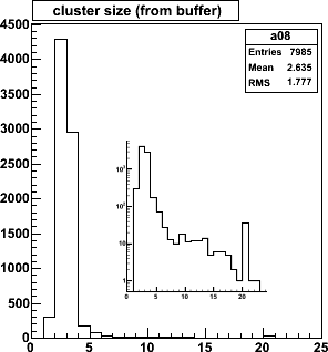
| Hits are clustered because of the track angles and the detector
tilt. Cluster sizes average 1.6 and 2.6, but there is a tail to large cluster
sizes, as shown in the inset (same plot, log scale). The cutoff at 20
is an artfact - my internal buffer size.
| 
| 
|
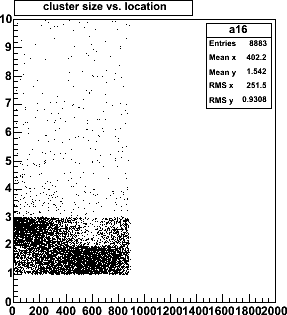
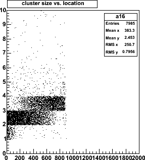
| The cluster size depends on the hit location. This is most easily seen
for the flat configuration (right), where there are clusters of size 1 at the
innermost strips, and clusters of size 3 further out at channel 880, 6.6cm
further out.
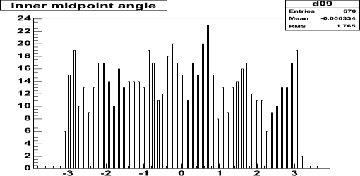
The left plot shows that tracks come in perpendicularly around strip
number 600, where 1-strip clusters are most prevalent, and 2-strip clusters
are more likely ar higher and at lower strip numbers.
| 
| 
|
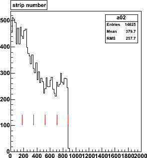
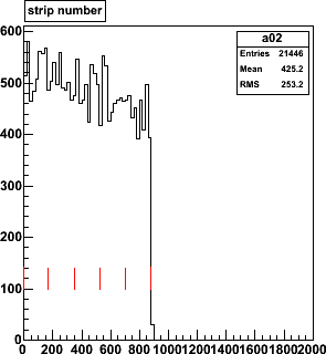
| Folding the track distribution with the cluster size distribution leads to
strip hit distribution, shown here for 9 AuAu events. For the flat planes,
the falling track density os compensated by the increasing cluster size.
On the left, you can see the dip at strip 600, where tracks are perpendicular.
| 
| 
|
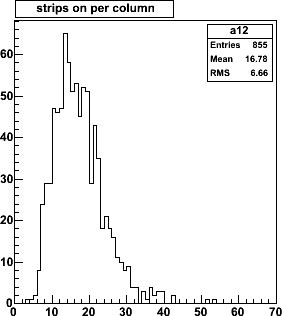
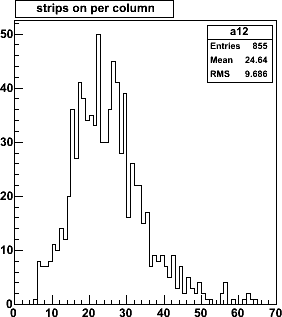
| Number of strip hits per column of ministrips for 9 events
(96 columns × 9 = 855 entries). Mean occupancies are 1.8% and 2.8%.
| 
| 
|
|
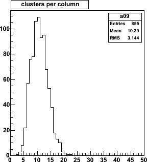
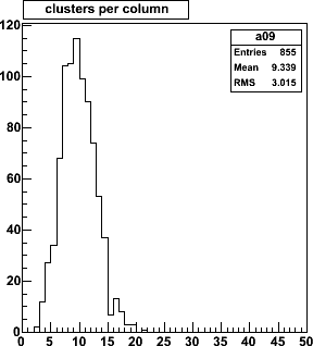
This is the distribution of clusters per ministrip column.
Typically there are 10 clusters distributed over 880 strips, which
is a 1.1% cluster density (~= track density).
Typically there are 1000 tracks (10.44× 96) hitting the first cone
in a central AuAu event.
| 
| 
|
|
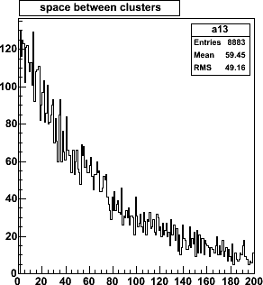
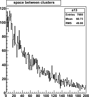
Distribution of empty space (counted in strips) between adjacent clusters.
An (extrapolated) separation of 0 strips means we have
merging or overlapping clusters. The probability of such merging clusters is
125/8883, or 110/7985 = 1.4%, the same for both configurations.
The pattern
recognition will have to deal with these (rare) overlap occurrences.
| 
| 
|
|
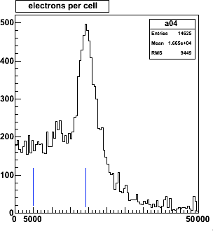
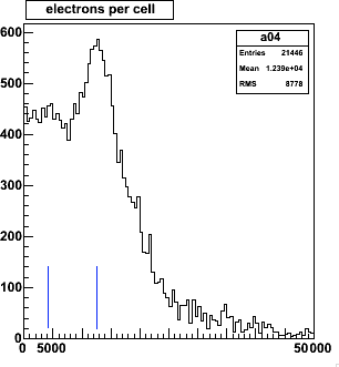
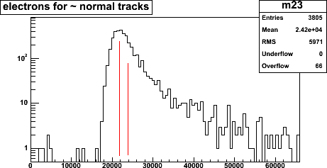
Electrons per strip hit, 17k and 12k respectively. A threshold cut is indicated,
at 1/4 of the most probable value: ~5000 and 4000 electrons, respectively.
| 
| 
|