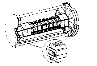
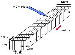
Each silicon sensor of each C-module is connected by a flexible kapton cable to its own front-end electronics printed-circuit board (Multi-Chip Module or MCM). The MCMs for each module (4 or 6 depending on which module) are supported inside a 4.26 x 3.1 x 5.32 cm Rohacell shell. These parallelepipedic modules populated by the MCM plates form two distinct plenum chambers. The two MVD plenum chambers are identical and made of 12 parallelepipedic Rohacell modules as shown in Figure 2. Only 4 out of the 12 modules are fully populated with MCMs. The fully populated modules (first and second module of each end) contain 6 equally spaced MCM plates as shown in Fig. 2, while all other modules contain 4 MCMs. The distance between the first MCM and the shell on either side is about 0.3 cm. Groves 0.2 cm deep are cut into the upper and lower sides of the Rohacell to maintain the MCMs in place.
Note that the 12 modules are held together by light axial pressure from the same end plates used for the C-modules.
The MCMs are the main heat source in the system
and dissipate about 2.5 W each. These electronics boards are thermally isolated
from the rest of the MVD by the foam shell and therefore are the only
components which need to be cooled down. The operating temperature of these
electronics must be maintained below 50 C. To achieve this, an air-cooling
system was selected.
The purpose of section 2 is to evaluate the airflow needed to cool these
components to the required temperature assuming a 2.5 W per MCM heat load.
Since the system is compact and the total heat load is relatively large, the
airflow velocity needed to maintain the MCMs at operating temperature will be
relatively high. In this case, vibrations may be induced by the air flowing
through the plenum which could shake the MCMs and cause the foam to fail. This
aspect of the problem will be discussed in section 3.
Sections 4 and 5 review the structure of the C-modules. Sagging of the C-module
assembly due to the axial compressive force applied to maintain the modules
together is considered in section 4. The MVD will operate in a relatively moist
environment (28% to 78% relative humidity). Due to large mismatch between the
Rohacell foam and the silicon strip moisture coefficients, high stresses are
expected in the foam due to hydroscopic effects. A finite element model for
the C-module assembly is used to predict stresses and displacements because of
moisture absorption is presented in section 5.
2.
Electronics cooling
As mentioned in section 1, the front-end electronics located in the two MVD
plenum chambers are a waste heat source in the system and dictate cooling
requirements. The performance of these electronics can be affected by high
temperatures which must be maintained below 50 C to insure proper functioning.
For design purposes, a maximum temperature of 40 C is used, which should allow
a reasonable safety margin. Air cooling was selected over water because of
lower-mass and convenience.
The purpose of this cooling study is to evaluate the velocity of the chilled air needed to maintain the MCMs below 40 C assuming a 2.5 W heat load per MCM. To evaluate the maximum temperature reached by the electronic chips on the MCMs, we need to look at three phenomena (see Fig. 3):
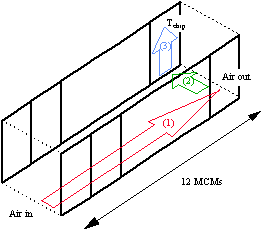
Tair = Tinlet + Q/v Ac Cp , (1)
where
Q is the total heat load from the inlet to d, is the air density, Cp is the
air specific heat, v is the airflow velocity and Ac is the channel
cross-section. If we assume a uniform heat load distribution along the channel,
the heat load from the inlet to d is given by
Q = (12) x (2.5 W) x (d/L), (2)
where L is the channel length (L = 12 x 53.2= 64.2 cm)
With these assumptions, the air temperature along the channel in the flow direction is a linear function of the distance from the inlet for a given airflow velocity. The air temperature along the channel for several airflow velocities is plotted in Fig. 4, assuming a 20 C inlet temperature. The outlet air temperature corresponds to the air temperature at the 12th module.
TMCM = Tair + QMCM/h AMCM , (3)
where QMCM is the heat load dissipated by one side of the MCM (i.e., 2.5/2 W), h is the heat transfer coefficient, AMCM is the MCM surface area exposed to air flow and QMCM/h AMCM is the temperature differential because of the MCM-to-air thermal exchange.
The heat transfer coefficient, h, can be evaluated from semi-empirical relations which depend on the flow regime (laminar or turbulent). For a laminar flow, this coefficient has been approximated by Sieder and Tate [1] as:
h = 1.86 (k/Dh) (Re Pr Dh/L)0.33, (4)
where k is the air thermal conductivity, Dh is the hydraulic diameter, Re the Reynolds number, Pr the Prandtl number and L the channel length. The Reynolds number Re is given by:
Re = v Dh/, (5)
where
v is the airflow velocity and is the air kinematic viscosity. In case of a
fully developed turbulent flow, Dittus and Boelter [2] give the following
relation:
h = 0.023 (k/Dh) (Re)0.8 (Pr)0.4 . (6)
Note that near the inlet, the thermal boundary layer is not fully-developed and, consequently the heat transfer coefficient is higher than given by Eq. (6). The resulting MCM temperature is lower than those predicted using a heat transfer coefficient for a fully developed flow. Therefore, using the coefficient given by (6) near the inlet is conservative.
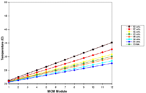
By combining eqs. (1) through (6), we can evaluate the temperature reached by the MCM plates along the channel. These temperatures are plotted in Fig. 5 for several airflow velocities.
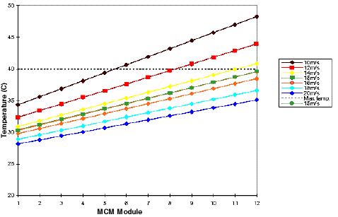
At any given airflow velocity, the average temperature reached by the plates is function of the air temperature along the channel since the temperature differential because of the MCM-to-air thermal exchange is constant. Therefore, for a given airflow velocity, the MCM temperature is a linear function of the distance from the inlet. Note that the MCM plate located at the outlet (module number 12) is the least cooled since the air flowing there is warmer. The dotted line in Fig. 5 indicates the maximum design temperature (40 C). The airflow velocity needed to maintain all MCMs below 40 C is at least 15 m/s. This airflow velocity produces an average heat transfer coefficient of 80.2 W/m2 C.
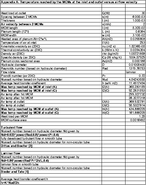
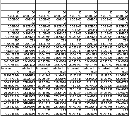
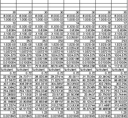
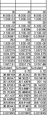
Using eqs. (1) through (6), we can also evaluate the average temperature reached by the MCMs located at the inlet and the outlet, as well as the temperature of the air at the outlet as a function of the airflow velocity. The spreadsheet used for these calculations is included in Appendix 2A.
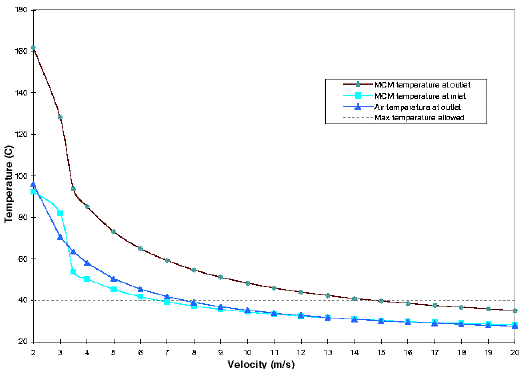
The blue curve with squares on Fig. 6 shows the temperature of the MCM at the inlet, while the red curve with circles shows the maximum temperature reached by any MCMs, i.e. the MCM temperature at the outlet. The air temperature at the outlet is shown by the red curve with triangles. The transition from laminar to turbulent flow occurs at an airflow velocity of about 3.5 m/s for this plenum geometry, and is shown in Fig. 6 by the vertical solid line. These results show again that an airflow velocity of at least 15 m/s is needed to maintain the MCMs at an average temperature of 40 C. The outlet air temperature corresponding to a 15 m/s airflow is 30 C for a 20 C inlet temperature.
Note that the slopes of the temperature curves are nearly flat and, therefore, MCM temperature is very sensitive to modeling errors for velocities in the 12 to 20 m/s range.
The temperature reached by one MCM plate given by eq. (3) is the average temperature of the MCM; this is the temperature that the MCM would reach if heat were spread uniformly. In eq. (3), we also assume that both sides of the MCM dissipate the same amount of heat, which is also function of the MCM design. It is therefore necessary to study the heat spreading across an MCM. An airflow velocity of 15 m/s is selected to perform the heat spreading study since a 15 m/s airflow is predicted to maintain all MCMs at an average temperature corresponding to the design temperature of 40 C.
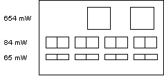
The silicon chips have different sizes and dissipate more or less heat as shown in Fig. 8. The chips located in the first, second, and third rows dissipate 0.654 W, 0.084 W and 0.065 W each, respectively, as shown.
A finite element model of the MCM plate was built using COSMOS/M to simulate a 15 m/s airflow and convective heat transfer on both sides of one MCM located at the outlet. The ambient air temperature was set to 30 C, which corresponds to the outlet air temperature computed in section 2.2. The average heat transfer coefficient was set to 80.2 W/m2 C, which corresponds to a 15 m/s airflow for the channel considered as computed in section 2.1.
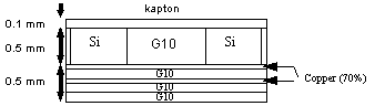
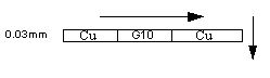
The finite element model contains 4 layers with different thermal conductivities: one kapton layer, one G10 layer where the silicon chips are embedded, one layer representing the 4 layers necessary to power the chips, and the bottom G10 layer. The two layers of G10 and the two layers of copper at 70% coverage are modeled as one single layer with equivalent conductivity in the plane direction and through the thickness. First, the thermal conductivity of the copper layer at 70% coverage shown in Fig. 9 needs to be computed in both direction using series and parallel models. In the plane direction, this layer can be viewed as one layer of G10 (30%) in series with one layer of Cu (70%). This in-plane equivalent conductivity Kin-plane is computed from the thermal conductivity of the copper layer kCu (= 400 W/mK) and the G10 layer kG10 (= 0.7 W/mK) as:
1/Kin-plane = 0.3/kG10 + 0.7/kCu = 0.4 (W/mK)-1, (7)
which corresponds to a thermal conductivity of 2.3 W/mK.
Through the thickness, this layer can be viewed as one layer of G10 in parallel with one layer of Cu and the equivalent conductivity Kthickness is given by:
Kthickness = 0.3 kG10 + 0.7 kCu = 280 W/mK. (8)
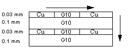
Then, the thermal conductivity in both directions of one layer of copper at 70% coverage and one layer of G10 shown in Fig. 10 can be evaluated using the same process. In the plane direction, these two layers are in parallel and the equivalent conductivity Keq plane is:
Keq plane = (0.03 Kthickness + 0.1 kG10)/0.130 = 1.1 W/mK. (9)
Through the thickness, the equivalent thermal conductivity Keq thickness is evaluated using a series model as:
1/Keq thickness = (0.03/Kthickness + 0.1/kG10)/0.130= 1.1 (W/mK)-1, (10)
which corresponds to a thermal conductivity of 0.9 W/mK.
The three other layers constituting the model are the kapton layer with a thermal conductivity of 0.2 W/mK, the G10 layer with a thermal conductivity of 0.7 W/mK, in which the silicon chips (with a thermal conductivity of 148 W/mK) are embedded, and the bottom G10 layer. Each silicon chip is associated with a volumetric heat source which corresponds to the heat it generates.
Temperature contours on both sides of the G10 layer containing the silicon chips (as shown by the arrows in Fig. 11) are shown in Fig. 12. The maximum average temperature on the MCM plate is 317 K (44 C), which agrees with the 40 C calculated by hand, but the maximum temperature is 326 K (53 C). This is not surprising since the temperature difference across the entire plate is 23 C.
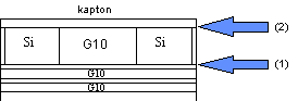

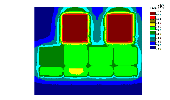
Fig. 12: Temperature distribution for the initial MCM design. Contour (1) is located at the interface of the G10 layer containing the silicon chips and the Cu layer. Contour (2) is at the interface between the same G10 layer and the kapton layer.
To decrease the temperature of the silicon chips, we need to spread the heat more uniformly across the MCM plate. To do so, we replace the 0.240 mm G10 layer by a 0.04 mm adhesive layer and a 0.200 mm aluminum plate. Temperature contours for this new design on both sides of the layer containing the chips (as shown by the arrows in Fig. 11) are shown in Fig. 13. The maximum temperature is now 316K (43 C), which is getting closer to the average temperature of 314 K (41 C) reached by the MCM. The temperature difference across the plate decreases to 6 C.
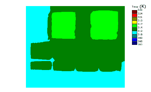
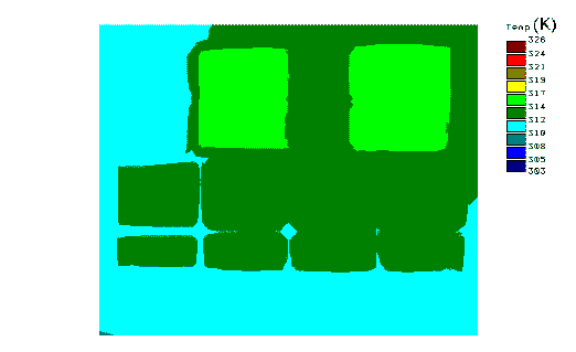
Fig. 13: Temperature distribution for the aluminum plate MCM design. Contour (1) is located at the interface of the G10 layer containing the silicon chips and the Cu layer. Contour (2) is at the interface between the same G10 layer and the kapton layer.
We try to reduce the temperature difference across the MCM even more by replacing the G10 layers and the aluminum plate by alumina substrates. Temperature contours on both sides of the alumina layer containing the silicon chips (as shown by the arrows in Fig. 11) for the alumina design are shown in Fig. 14. The maximum temperature reached by the MCM is 315 K (42 C) and the temperature difference across the plate is 5 C. With this last design, we only decrease the temperature of the chips by 1 C more than the aluminum plate design (316 K with the aluminum versus 315 K with alumina). This very small gain is not justified since the alumina design is much more expensive.
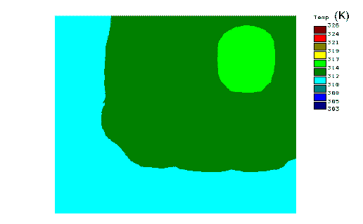
Fig. 14: Temperature distribution for the alumina substrate MCM design. Contour (1) is located at the interface of the alumina layer containing the silicon chips and the second alumina susbstrate. Contour (2) is at the interface between the alumina layer with the chips and the kapton layer.
The magnitude of the heat flux on both sides of the MCM plate is plotted in Fig. 15 for the initial design and the aluminum plate design. The top surface (see Fig. 15) designates the top of the kapton layer, while the bottom face (see Fig. 15) designates the other side of the MCM plate (i.e., the G10 layer for the initial design and the aluminum plate for the modified design).
The heat flux distribution is similar to the temperature distribution since the heat flux is equal to the temperature difference between the air and the MCM plate times the average heat transfer coefficient. For both designs, the heat flux is similar on both sides of the MCM plate. However, for the aluminum plate design, the heat flux is much more uniform.
To decrease the MCM temperature, we need to reduce the heating of the air along
the plenum, and increase the MCM-to-air thermal exchange and the heat
spreading. The heating of the air along the plenum can be decreased by
modifying two parameters, the massflow rate or the inlet temperature. By
increasing the massflow rate, we can lower the temperature rise of the air
flowing through the plenum. If increasing the airflow velocity is not
acceptable, since airflow induced vibrations are a concern, the massflow rate
can be increased without changing the airflow velocity by increasing the MCM
spacing. The maximum temperature reached by the MCMs versus the MCM spacing for
a 15 m/s airflow are plotted in Fig. 16.
The maximum temperature decreases slowly when the spacing between the MCM
plates increase. Because of space limitations, it is necessary to keep the MVD
plenum chamber as small as possible, and it is not acceptable to choose a MCM
spacing greater than 8 mm. By increasing the spacing from 6 mm to 8 mm, the
maximum temperature reached by the MCM decreases from 39.5 C to 37.5 C. This
is a small gain compared to the gain we can achieve by lowering the temperature
of the air at the inlet. The air temperature level along the plenum is directly
function of the air temperature at the inlet. Using cooler air at the inlet
directly lowers the maximum temperature reached by the MCMs.
The heat transfer between an MCM plate and the air is another parameter we can
influence. To increase the MCM-to-air thermal exchange, we would need to
increase the heat transfer coefficient by increasing the airflow velocity.
However, this may not be acceptable since flow induced vibrations are a
concern.
The last parameter is the heat spreading across the MCM plate. With the
aluminum plate design, the temperature difference across the plate is only 6 C
(compared with 23 C for the initial design). Therefore, the heat spreading can
not be improved and has been taking care of. The maximum temperature reached by
the MCM has been decreased considerably by adding an aluminum plate to spread
the heat uniformly. This change in design decreased the maximum temperature
from 56 C to 43 C. Increasing the MCM spacing does not decrease much the
temperature; only 2 C are gained when the MCM spacing is increased from 6 mm
to 8 mm. The inlet air temperature represents a direct gain on the maximum
temperature reached by the MCM and is the most efficient way to decrease the
MCMs temperature without increasing the airflow velocity because of vibration
concerns.
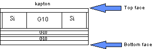
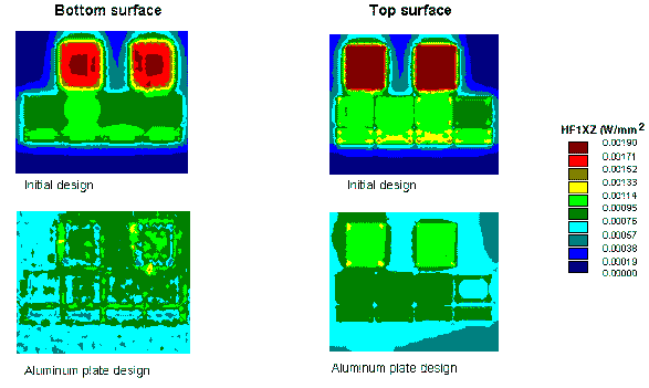 Fig. 15: Heat flux contours for the initial and the aluminum plate design. The
top surface of the MCM designates the top of the kapton layer, while the bottom
surface designates the other side of the MCM.
Fig. 15: Heat flux contours for the initial and the aluminum plate design. The
top surface of the MCM designates the top of the kapton layer, while the bottom
surface designates the other side of the MCM.
2.4.
MCM cooling summary
The maximum temperature reached by the MCM is the result of three heat transfer
phenomena: the heating of the air as it moves through the plenum, the
MCM-to-air thermal exchange and the heat spreading. All 3 phenomena depend on
the system heat load. The heating of the air is function of the massflow
through the plenum. The MCM-to-air thermal exchange essentially depends on the
heat transfer coefficient of the MCM plate, which is directly related to the
airflow Reynolds number. Finally, the heat spreading across the MCM plate
depends on the conductivities of the different materials constituting the MCM
plate, i.e., on the MCM design. 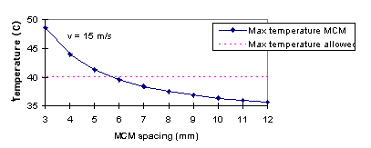
References