Another method used to find the vertex is based on "pseudo-tracking." This method treats all pairs of hits in the inner and outer barrels as potential tracks and calculates a vertex position from them. The real vertex appears as the most probable value of the vertex position.
Figure 6: Probability vs. the difference in the parallel
strip in the outer
barrel which was hit and the strip that would have been hit with
no multiple scattering. All charged particles which hit both barrels
are included.
There are two stages in the pseudo-tracking vertex search. First, only the
parallel strips are used, obviating the need to test all pairs of hits as each
parallel strip covers a small
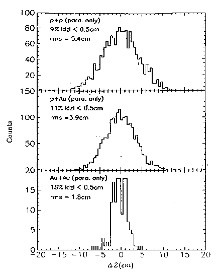
Because the peak found using pseudo-tracking with parallel strips is broad,
the vertex position is estimated by taking the center of gravity of three bins
around the maximum. Because the strips are long (5cm) in the z direction, this
method can not give very good vertex resolution. Fig. 8 shows the vertex
resolution for p+p, p+Au, and Au+Au using pseudo-tracking with parallel strips
only. For p+p and p+Au, this method gives better resolution than the center of
(CG) and is much less noise sensitive. However, pseudo-tracking
with parallel strips alone still does not give a vertex resolution for p+p
which is significantly better than the variation in the vertex position
itself5.
Figure 8: The vertex resolution using pseudo-tracking with parallel
strips only for p+p, p+Au minimum bias, and Au+Au central. The horizontal axis
is the difference the true vertex and the vertex found.
This first stage using parallel strips is used to estimate a vertex
position. The second stage of the vertex search uses perpendicular strips which
are short in the z direction (100
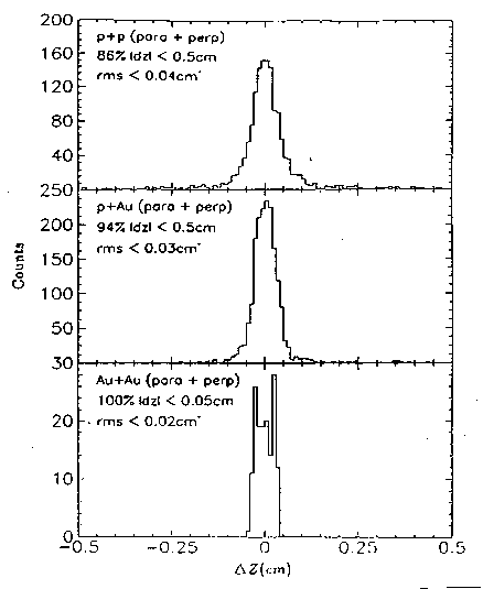
Figure 9: Notice the difference in scale from fig. 8.
The vertex resolution using pseudo-tracking with both
parallel and perpendicular
strips for p+p, p+Au minimum bias, and Au+Au central.
*Due to the bin size used, the RMS deviations are upper limits.
Fig. 9 shows the vertex resolution using both stages of pseudo-tracking.
The correct vertex is found in all events tested for central Au+Au collisions.
For p+p and Au+Au the correct vertex is usually found. Table 3 summarizes the
efficiency of pseudo-tracking vertex search for different assumed levels of
noise for the three systems. "Total events" and "triggers" are the total
number of Monte Carlo events and the number of those that satisfied the
"trigger" condition - at least two charged particles hitting both cylinders
of the vertex detector. The column labeled "% of triggers" gives the
efficiency of the vertex search algorithm - the fraction of the events for
which the vertex found was within 5mm of the true vertex. The last column gives
the resolution of the vertex finding algorithm based on the widths of the peaks
in fig. 9. These widths are upper limits due to the size of the bins used in
the pseudo-tracking algorithm. Especially for p+p collisions, noise has a
significant effect on the vertex finding efficiency.
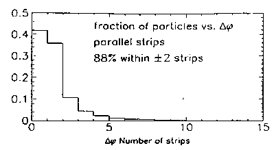
 (azimuthal angle). Particles from
the central axis of the vertex detector have the same
(azimuthal angle). Particles from
the central axis of the vertex detector have the same  at each barrel,
except for small variations due to multiple scattering. Fig. 6 shows a
distribution of the change in the strip number hit in the outer barrel due to
multiple scattering in the inner barrel; most particles hit the outer barrel
within
at each barrel,
except for small variations due to multiple scattering. Fig. 6 shows a
distribution of the change in the strip number hit in the outer barrel due to
multiple scattering in the inner barrel; most particles hit the outer barrel
within  2 strips of the expected position. For each hit in the outer
barrel, all hits in the inner barrel which are within 2 strips are used
to calculate a possible vertex position. The top part of fig. 7 shows the
resulting distribution of vertices for a sample Au+Au event. An estimate of the
event vertex appears as a peak. The peak height gives the number of particles
hitting both barrels of this half of the detector. The background comes from
random pairs of hits. Limiting the hits tested to 2 strips reduces the
number of pairs that must be tested by a factor of
2 strips of the expected position. For each hit in the outer
barrel, all hits in the inner barrel which are within 2 strips are used
to calculate a possible vertex position. The top part of fig. 7 shows the
resulting distribution of vertices for a sample Au+Au event. An estimate of the
event vertex appears as a peak. The peak height gives the number of particles
hitting both barrels of this half of the detector. The background comes from
random pairs of hits. Limiting the hits tested to 2 strips reduces the
number of pairs that must be tested by a factor of  =
=
 . This reduces the background in the histograms shown
in the upper half of fig. 7 by while only reducing the counts
in the peak by about 12% (see fig. 6).
. This reduces the background in the histograms shown
in the upper half of fig. 7 by while only reducing the counts
in the peak by about 12% (see fig. 6).
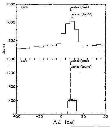
Figure 7: Au+Au - pseudo-tracking example. Top shows the distribution of
vertices using parallel strips only.
Bottom shows the distribution of vertices using the
perpendicular strips.
Arrows mark the true vertex and
the vertex found in each stage.
 ), and determine the vertex much more
accurately. Beginning with an approximate vertex reduces the range of vertex
positions to be searched and increases the speed of the algorithm. The second
stage of the vertex search is similar to the first, but as each perpendicular
strip occupies a large , the number of pairs of hits that must be
tested is about N1N2/3, where 3 is the number of different azimuthal
segments with perpendicular strips and N1and N2 are the number of hits
on the perpendicular strips in the inner and outer barrels, respectively. For
central Au+Au events, this number is large, so the algorithm is slow. The
vertex from the first stage of pseudo-tracking is used to restrict the pairs of
strips which are tested; for Au+Au, only those pairs of strips which point to a
vertex position within 5cm of the vertex found in the first stage of
pseudo-tracking are tested. For p+p and p+Au, this range is expanded to 10cm. A histogram of vertex positions is calculated from the pairs of hits. An
example of one of these histograms is shown on the bottom part of fig. 7. The
vertex position appears as the peak in this distribution.
), and determine the vertex much more
accurately. Beginning with an approximate vertex reduces the range of vertex
positions to be searched and increases the speed of the algorithm. The second
stage of the vertex search is similar to the first, but as each perpendicular
strip occupies a large , the number of pairs of hits that must be
tested is about N1N2/3, where 3 is the number of different azimuthal
segments with perpendicular strips and N1and N2 are the number of hits
on the perpendicular strips in the inner and outer barrels, respectively. For
central Au+Au events, this number is large, so the algorithm is slow. The
vertex from the first stage of pseudo-tracking is used to restrict the pairs of
strips which are tested; for Au+Au, only those pairs of strips which point to a
vertex position within 5cm of the vertex found in the first stage of
pseudo-tracking are tested. For p+p and p+Au, this range is expanded to 10cm. A histogram of vertex positions is calculated from the pairs of hits. An
example of one of these histograms is shown on the bottom part of fig. 7. The
vertex position appears as the peak in this distribution.
| system | Pnoise | Total events | Triggers | % of triggers |  (mm) (mm) |
|---|---|---|---|---|---|
| p+p | 0.0001 | 2000 | 1699 | 91% |  0.4 0.4 |
| p+p | 0.0003 | 2000 | 1699 | 86% | 0.4 |
| p+p | 0.0010 | 2000 | 1699 | 71% | 0.4 |
| p+Au | 0.0001 | 2000 | 1921 | 97% | 0.3 |
| p+Au | 0.0003 | 2000 | 1921 | 94% | 0.3 |
| p+Au | 0.0010 | 2000 | 1921 | 90% | 0.3 |
| Au+Au | 0.001 | 150 | 150 | 100% | 0.2 |
Table 3: Efficiency of pseudo-tracking vertex search vs. assumed level
of noise for p+p, p+Au, Au+Au. Interaction diamond assumes
 = 5.7, 16, 20cm for p+p, p+Au, Au+Au, respectively.
See text for explanation of columns.
= 5.7, 16, 20cm for p+p, p+Au, Au+Au, respectively.
See text for explanation of columns.
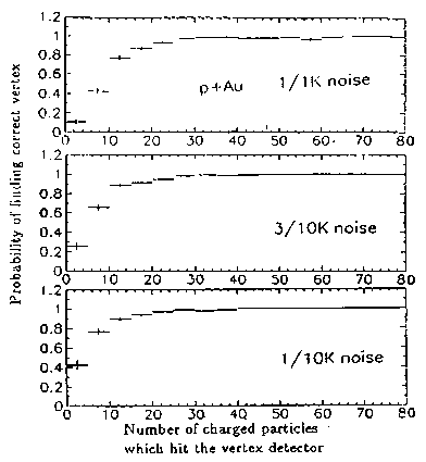
Figure 10: p+Au minimum-bias events from Fritiof. The probability that the correct vertex will be found vs. the number of charged particles that hit both layers of the vertex detector for three assumptions about the noise level. Notice the differences in efficiency for the lowest multiplicity, where the effects of noise are most important
Fig. 10 demonstrates one source of problems with the pseudo-tracking
vertex search --- when the multiplicity is very low, the probability of finding
the vertex is also low and this probability gets smaller for higher noise
levels. Higher noise levels have a significant effect on the vertex finding
efficiency at low multiplicity (below  10), but the efficiency reaches
100% in each case for sufficiently high multiplicity. In an ideal
case, with no noise, 100% efficiency, and no multiple scattering, the
algorithm would work for even one charged particle hitting both layers of the
detector.
10), but the efficiency reaches
100% in each case for sufficiently high multiplicity. In an ideal
case, with no noise, 100% efficiency, and no multiple scattering, the
algorithm would work for even one charged particle hitting both layers of the
detector.
| system | Pnoise | Total events | Triggers | Vertex correct | % of Triggers |
|---|---|---|---|---|---|
| p+p | 0.0003 | 2000 | 1699 | 1228 | 72% |
| p+Au | 0.0003 | 2000 | 1921 | 1662 | 87% |
| Au+Au | 0.001 | 150 | 150 | 150 | 100% |
Table 4: Efficiency of pseudo-tracking vertex search
for p+p, p+Au, Au+Au with only 2 azimuthal segments of perpendicular strips
used and a length of 64cm. Interaction diamond assumes
= 5.7, 16, 20cm for p+p, p+Au, Au+Au, respectively.
Compare this to table 4, using the full detector.
A vertex detector like the one described in the Tales/Sparhc letter of
intent7 which had only 2 azimuthal segments of strips perpendicular to the
beam, instead of 3, and was 64 cm long, instead of 100cm, could still find the
vertex, but with reduced efficiency. Table 4 shows the expected vertex finding
efficiency for this detector configuration. The efficiencies are smaller
(compare to table 3), especially for p+p, but if the cost savings are large
enough, the efficiency loss may be acceptable. Some efficiency is lost when the
vertex is outside the shorter detector. However, tests with the full detector
configuration show that the pseudo-tracking algorithm can find the vertex in
central Au+Au collisions in 94 out of 100 events even when it is 50cm outside
of the detector (100cm from the center of the detector), although the
resolution falls to 2mm.