| (1) The problem is this: there is a bundle of light-emitting fibers, spread over a 20×20 mm square area, and a 3×3 mm avalanche photodiode (APD) for the detection of this light. | 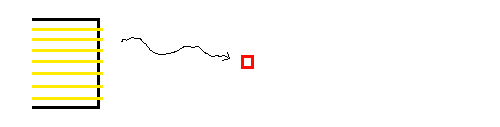
|
| (2) Plan B: Each fiber produces a pretty wide cone of light. | 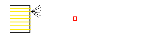
|
| (3) If we place in front of each fiber a small lens, we can make all rays come out parallel. | 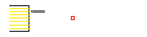
|
| (4) Now we can make the magnifying lens less extreme, and obtain a small image. | 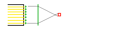
|
| (5) ... as shown here in the Geant model (lens: r1=40mm, r2=60mm, a0=-0.005, not optimized ) | 
|
|
(6) This shows a fiber (red), spraying rays in ±30°. These rays are
intercepted by a microlens, which turns them into parallel rays, which are then
sent to the detector by the big imaging lens.
Here the little lens is not so small, but the concept scales exactly. Also note that since the rays leaving the microlenses are parallel, the imaging lens can be moved all the way to the left, saving space. In addition, the imaging lens can be optimized to shorten the focal length. | 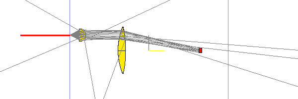
|
| (7) So an array of microlenses, matched to the fiber matrix, plus a simple acrylic lens gets (almost) all the photons onto the detector. | 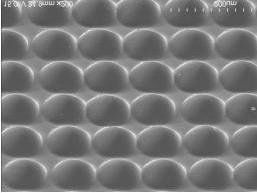
|
|
(8) Caveats: the solution modeled in (6) works because the rays are thrown from
a single point. This is an approximation. In reality, it depends on the ratio
of the fiber diameter to the fiber spacing. If this is <<1, the approximation
holds.
Pictured is a piece of the prototype calorimeter. I use that below to simulate the fiber size. | 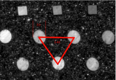
|
| (9) Make an array of sperical (can be tuned later) lenses | 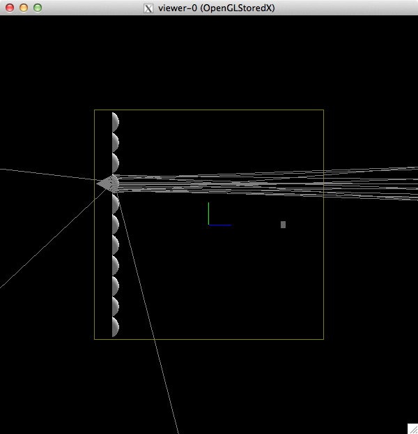
|
| (10) Note that if you back each lens with a cylinder, the spread of the rays from the end of the fiber is reduced. In addition, the lens array is now coupled directly to the fibers, with a dab of optical grease. This eliminates surface losses at this interface. | 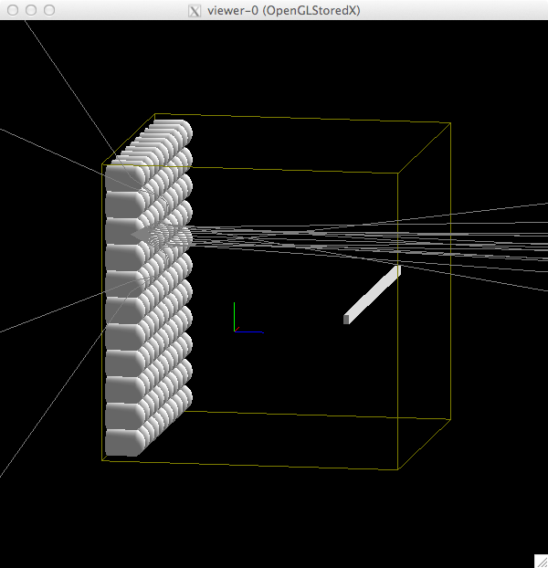
|
| (11) Simulate rays from fibers at different positions | 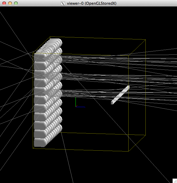
|
| (12) Now that we have a bunch if parallel ray bundles, we can try to focut these. This is an acrylic lens, and it cannot do the job. | 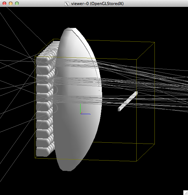
|
| (13) Back to the lens array for a bit. Before, we had separate, tangent cylinders. These have been expanded so there is a single block. | 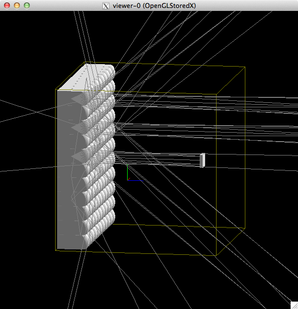
|
| (14) Grab the fresnel lens from the Cherenkov detector. Needs some tuning | 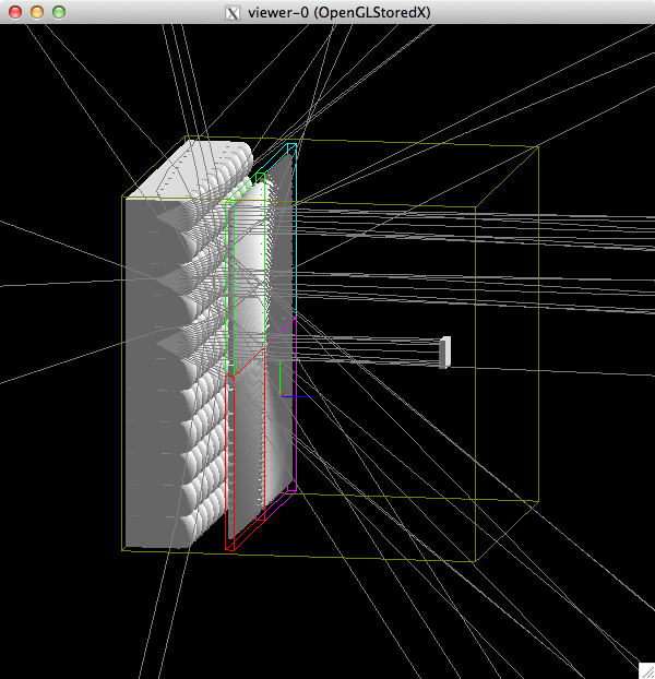
|
| (15) The Fresnel is tuned to focus parallel rays onto the detector. Note how thick the fresnel lens now is - more on this later. | 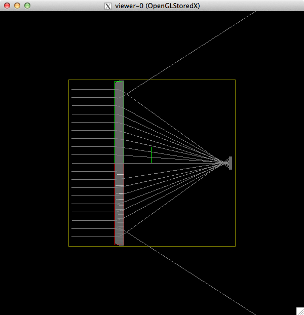
|
| (16) Put the lenslet array back. Looks good. The number of generated rays is 3×20. Stray rays number 32. So we have about 50% efficiency. In this picture, the angular distribution was uniform in y, and zero in x. The upper and lower parts of the cones are not intercepted by the lenslet, leading to the losses. | 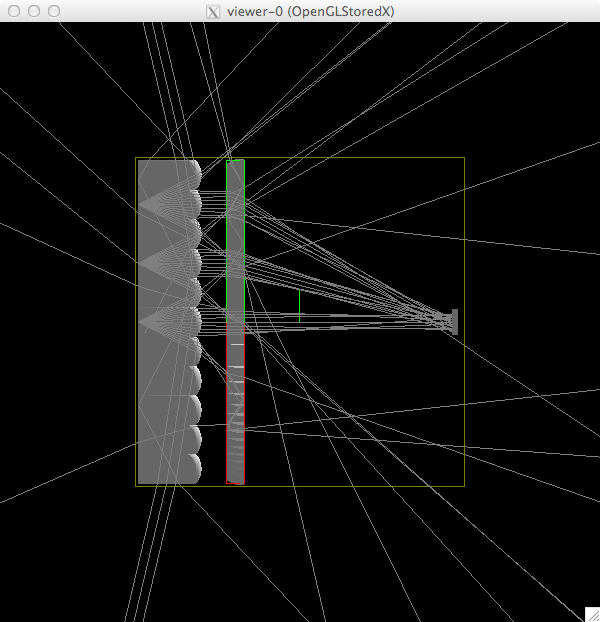
|
| (17) Add the finite fiber diameter, taken from the photo in (8). The starting positions of the photons is uniform across a small circle. The angular distribution here is gaussian in x and y, with a small sigma. We need to pin down what the actual starting distribution is. | 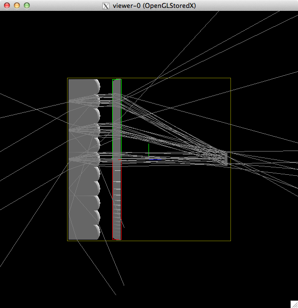
|
| (18) | 
|
| (19) | 
|
Hubert Van Hecke Last modified: Tue Oct 6 15:38:40 MDT 2020