| |
| postscript |
The histogram is fit with the function T=A*exp(-C*L/lamda**4). This expression reflects the probability that a photon of wavelength lamda is NOT Rayleigh-scattered when traversing a block of length L. A is an overall normalization constant, and C is a constant of the material, describing the 'clarity' or transpancy of the aerogel. C is to first order independent of the index of refraction, and depends mostly on process control variables during the production of the aerogel.
On the figure are also shown curves that predict the transmission spectra for samples of the same material (same A and C), but of different thicknesses. Note that a 5mm sample would have plenty of transmission at 350nm.
|
The figure on the right shows the (simulated) spectrum of initially produced
cherenkov photons, fit to 1/lambda**2. The short wavelengths dominate. On the
right this spectrum is separated into 2 components: photons that are scattered
before they exit the aerogel (black histogram), and those that exit without
scattering (yellow), for 3 different values of the clarity.
[For reference, the bottom value 0.0200 is typical for hygroscopic aerogel from Airglass in Lund, and the middle value 0.0100 is typical for the hydrophobic aerogel from Matsushita. The top value 0.0050 is again a factor of 2 better, but purely hypothetical so far]. Note that the unscattered photons are not at all absent at short wavelengths, even below 200nm.
|
|
| postscript |
|
The picture on the right plots the number of unscattered photons vs their
position of origin in the aerogel. z=0 means they are produced where the
particle enters, and therefore they have to traverse the whole 3cm block
before emerging unscattered. Those produced close to z=3cm can get out almost
immediately. Note that unscattered photons predominatly come from close to the
exit face of the block, and are dominated by short wavelengths.
|
|
 The MC used above was verified in a series of beam tests
[2] using the test fixture shown here. The beam enters
from the left, and enters the cubical sample compartment, where the aerogel is
held. Light is reflected off a 15cm spherical mirror. Cherenkov rings are
formed in the focal plane.
The MC used above was verified in a series of beam tests
[2] using the test fixture shown here. The beam enters
from the left, and enters the cubical sample compartment, where the aerogel is
held. Light is reflected off a 15cm spherical mirror. Cherenkov rings are
formed in the focal plane.
The back part of a Polaroid camera can be mounted such that the film plane coincides with the focal plane of the mirror. In this arrangement, one can make direct color photos of the cherenkov rings.
In a second configuration, a fresnel lens is placed in the focal plane and light is directed
onto a 2" PMT. In this arrangement, we can do photon counting using a small
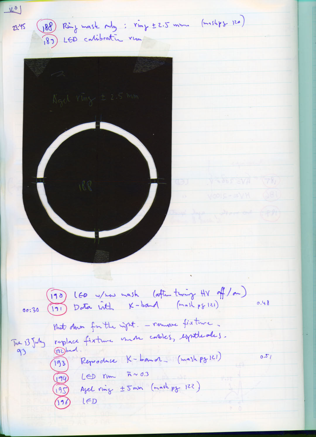
PMT. By taping black paper masks onto the fresnel lens, we can block areas of
the focal plane and count photons in the cerenkov ring, in the inside area
etc.
In a third arrangement (not shown), a scope camera (B/W polaroid) can be mounted such that the film plane is in the same place as the PMT face, in order to photograph the cherenkov image spots [4].
|
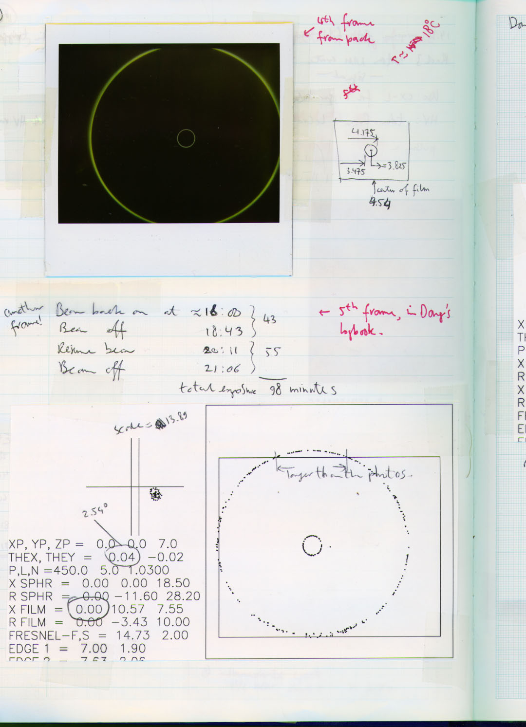
| Picture taken with Airglass aerogel, n=1.030. The small white ring in the center is from cherenkov ligh produced as the 450 GeV/c proton beam travrsing the air between the aerogel and the sperical mirror. The horizontal offset is caused by a 2.54° rotation of the apparatus w.r.t. the beam. | 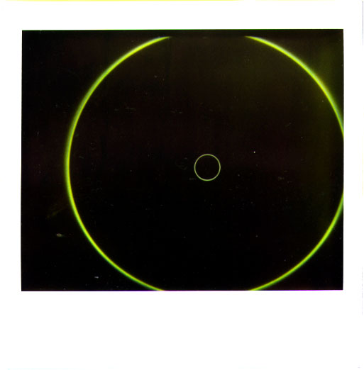
|
| Picture taken with KEK aerogel, n=1.010. It takes about 100 minutes for such an exposure. | 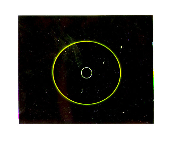
|
| B/W polaroid taken in the 'spot image plane' [4], which is where the PMT face would be. | 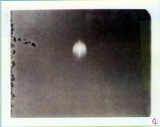
|
Absorption in aerogel?Using the photographs to verify the size and location of the cherenkov rings, masks were cut in order to count how many photons are in the ring, in the little air ring, and in the area in between the rings. There was good quantitative agreement between the MC predictions for all cases and the measurements made. In the MC, only Rayleigh scattering was taken into account, and no absorption was assumed.One reason to ignore absorption is that transmission spectra at different thicknesses always give good agreement with fits to T=P1*exp(-P2*T/lambda**4), where T is the sample thickness, and P2 is a property of the material, P1 is an overall normalization. Note that the P2's are almost the same in the two fits, and that the P1's can be interpreted as being due to a uniform loss of about 1.5% per cm, independent of wavelength. |
|
 The curves show the transmission spectra for the same aerogel, but for
different sample thicknesses, taking into account only Rayleigh scattering,
plus a uniform loss of 1.5% per cm. That is, there is no frequency-dependent
absorption.
The curves show the transmission spectra for the same aerogel, but for
different sample thicknesses, taking into account only Rayleigh scattering,
plus a uniform loss of 1.5% per cm. That is, there is no frequency-dependent
absorption.
Clearly a measurement of a 105mm-thick sample can tell us nothing about absorption below 500nm.
To measure the effect of absorption at 700nm, the sample has to be thin enough so that Rayleigh losses are minimal. 20-50mm is probably thin enough.
In order to measure absorption at 300nm, a sample of 2mm or thinner needs to be cut.
System spectral responseIf you want to take advantage of the large amount of blue light available, you have to choose a blue-sensitive PMT. These spectra are taken from the EMI catalog, and show the quantum efficiency for 3 different type of photocathodes. |
|
| The materials used in the system need to be matched to the chosen PMT
response spectrum. Just about all papers and plastics cut off around 270 nm,
but Aluminum has a flat response all the way across.
[5]
One should consider using aluminum foil or aluminized mylar for a reflector, and let the aerogel do the randomizing, since it has reflective properties superior to the best Tyvek (labeled 'total'). Either that or obtain Spectralon. |
|
| 
| 
|
| Absorption: | Emission: |
| 
|
| postscript | postscript |
|
 The picture on the left shows the trajectory of the photons, for a beam
particle incident from the left into a 3-cm block of n=1.02 aerogel. The
forward cone is clearly visible.
The picture on the left shows the trajectory of the photons, for a beam
particle incident from the left into a 3-cm block of n=1.02 aerogel. The
forward cone is clearly visible.